Thermal EMF Measurement and Seebeck Effect Experiment

Determination of Thermal EMF

Experiment: Plotting the Temperature vs. EMF Diagram Using a Potentiometer

Department of Physics | Undergraduate Laboratory

Objective of the Experiment

To understand the principle of the Seebeck Effect.

To calibrate a thermocouple (e.g., Copper-Constantan) using a potentiometer.

To plot the calibration curve: Temperature Difference (θ) vs. Thermo-EMF (E).

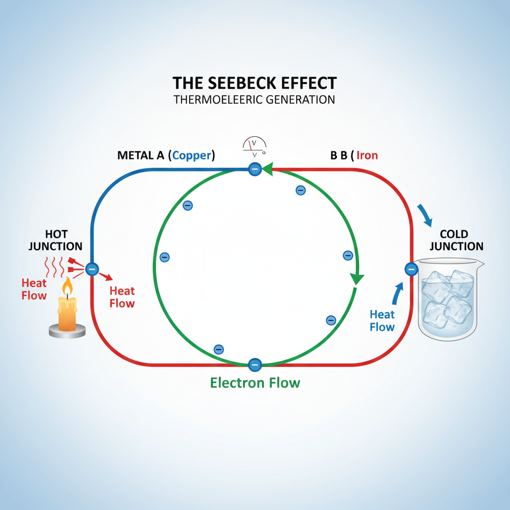
Theory: The Seebeck Effect

When two dissimilar metals are joined to form a closed loop and the two junctions are maintained at different temperatures, an electromotive force (EMF) is induced. This is known as the thermal EMF.

E = aθ + bθ²

Where 'E' is the thermo-EMF, 'θ' is the temperature difference between hot and cold junctions, and 'a' and 'b' are constants depending on the metals.

Experimental Apparatus

Potentiometer (Measurement Device)

Thermocouple (Copper-Constantan or Chromel-Alumel)

Sensitive Galvanometer & Jockey

Stable DC Source (Battery Eliminator/Accumulator)

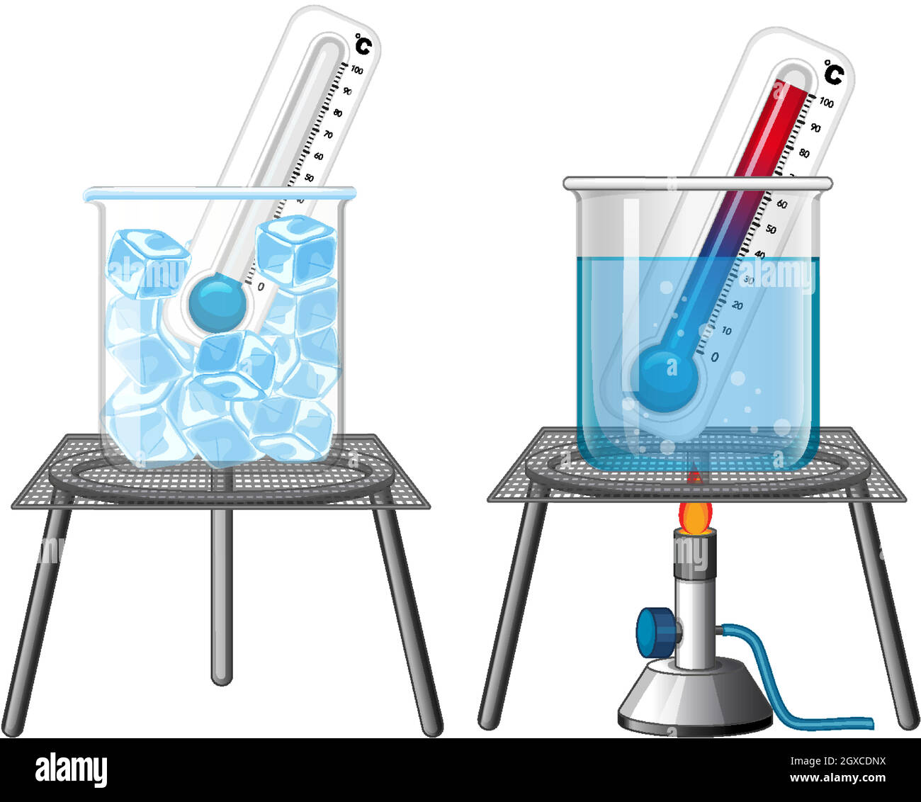
Two Beakers (Ice Bath & Sand/Water Bath) + Thermometers

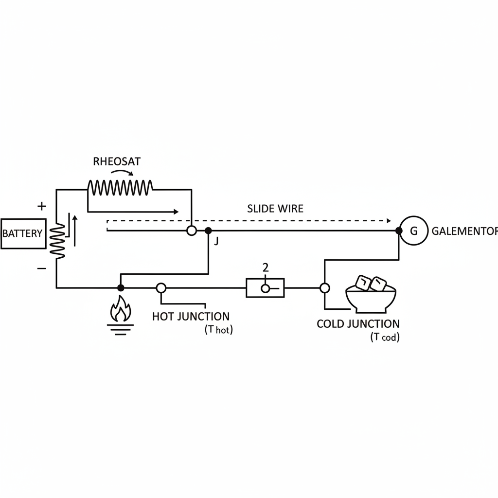
Circuit Diagram

The potentiometer measures the small EMF generated by the thermocouple without drawing current (Null Method). The cold junction is kept at 0°C (Ice), and the hot junction is heated gradually.

Procedure: Initial Setup

1. Cleaning: Clean the ends of the thermocouple wires with sandpaper to ensure good electrical contact.

2. Junction Placement: Immerse one junction in a beaker of melting ice (Cold Junction at 0°C) and the other in a beaker of water/oil (Hot Junction).

3. Standardization: Connect the standard cell to the potentiometer and adjust the rheostat to standardize the wire (e.g., potential gradient k).

Procedure: Measurement

Heat the hot junction beaker slowly using a bunsen burner or electric heater.

For every 5°C or 10°C rise in temperature, insert the key and balance the potentiometer (find the null point length 'l').

Calculate EMF (E) using E = k × l (where k is the potential gradient). Record readings until water boils (~100°C).

Observation Table Format

Temp of Cold Junction (°C)

Temp of Hot Junction (°C)

Temp Diff θ (°C)

Balancing Length l (cm)

Thermal EMF E = kl (mV)

Results: Temperature vs. EMF Diagram

The graph plots Temperature Difference (X-axis) against the measured Thermal EMF (Y-axis). For lower temperature ranges (0-100°C), the relationship is approximately linear.

Results & Discussion

Linearity: The graph shows a nearly straight line passing through the origin, indicating that EMF is directly proportional to temperature difference (E ∝ θ) for this range.

Slope: The slope of the graph (dE/dθ) gives the thermoelectric power (Seebeck Coefficient) of the thermocouple pair.

Neutral Temp: Within the 0-100°C range, the neutral temperature (where EMF peaks) is not reached for Cu-Constantan, hence no parabolic curve is observed.

Precautions and Sources of Error

• Keep the cold junction exactly at 0°C; replenish ice as needed.<br>• Ensure tight connections to minimize contact resistance.<br>• Stir the hot water bath continuously for uniform temperature measure.<br>• Avoid parallax error while reading the potentiometer scale.

Conclusion

The thermal EMF was successfully determined for various temperatures. The Temperature vs. EMF diagram was plotted, verifying the Seebeck effect characteristics for the given thermocouple.

Thank you.