

Geospatial Foundation Models for Agriculture & Environment
Explore how large-scale AI foundation models like NASA's Prithvi are transforming geospatial science, precision agriculture, and environmental monitoring.
Foundation Models for Geospatial Analysis
Agriculture & Environmental Studies
A lecture for university students on how large-scale AI models are transforming geospatial science
We recognise and pay respect to the Elders and communities – past, present, and emerging – of the lands that the University of Sydney's campuses stand on. For thousands of years they have shared and exchanged knowledges across innumerable generations for the benefit of all.
Lecture Outline
Topics covered today
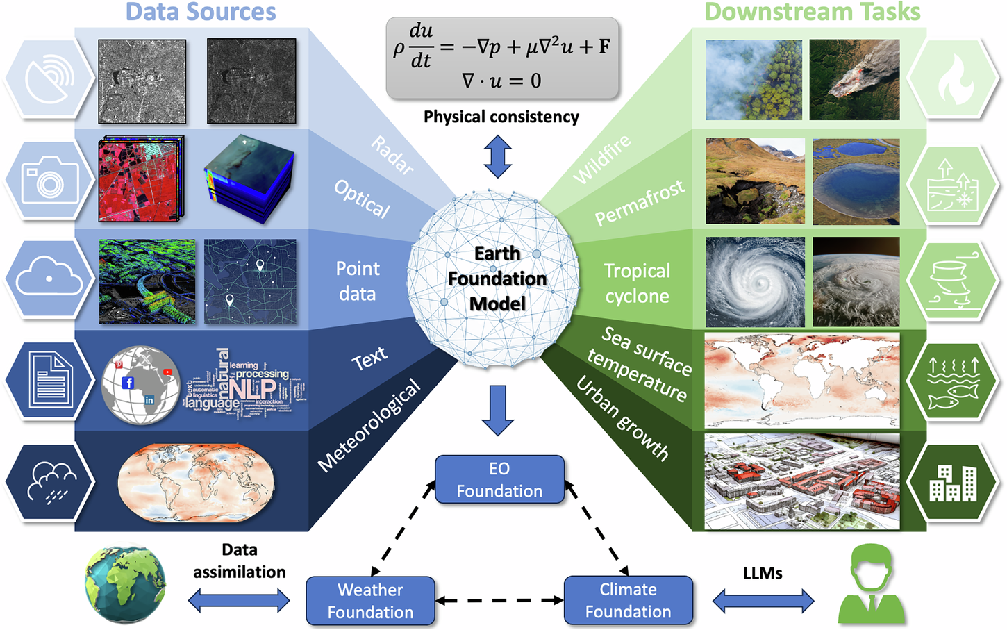
What are Foundation Models?
Geospatial Data & Remote Sensing
Foundation Model Architectures
Applications in Agriculture
Applications in Environmental Studies
Key Models & Benchmarks
Case Studies & Real-world Deployments
Challenges, Limitations & Future Directions
What are Foundation Models?
Large-scale pre-trained AI models adaptable to many tasks
Trained on massive, diverse datasets using self-supervised learning
Can be fine-tuned for specific downstream tasks with minimal labelled data
Examples: GPT, BERT, ViT — now extended to geospatial/remote sensing data
Enable transfer learning across domains: images, time-series, multi-modal data
Reduce the need for large task-specific labelled datasets
Particularly powerful where labelled geospatial data is scarce or expensive
Foundation
Model
Crop Mapping
Flood Detection
Land Use
Soil Analysis
Climate Monitoring
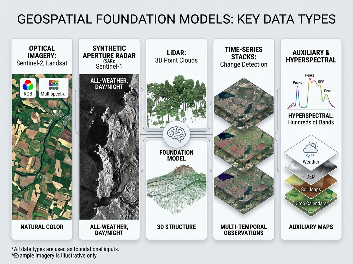
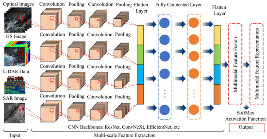
Geospatial Data & Remote Sensing
Types of data used in geospatial foundation models
Optical imagery: Sentinel-2, Landsat, Planet (multispectral, RGB)
Synthetic Aperture Radar (SAR): Sentinel-1 — all-weather, day/night
LiDAR: 3D point clouds for terrain, canopy structure
Hyperspectral: Hundreds of narrow spectral bands
Time-series stacks: multi-temporal observations for change detection
Auxiliary: weather, DEM, soil maps, crop calendars
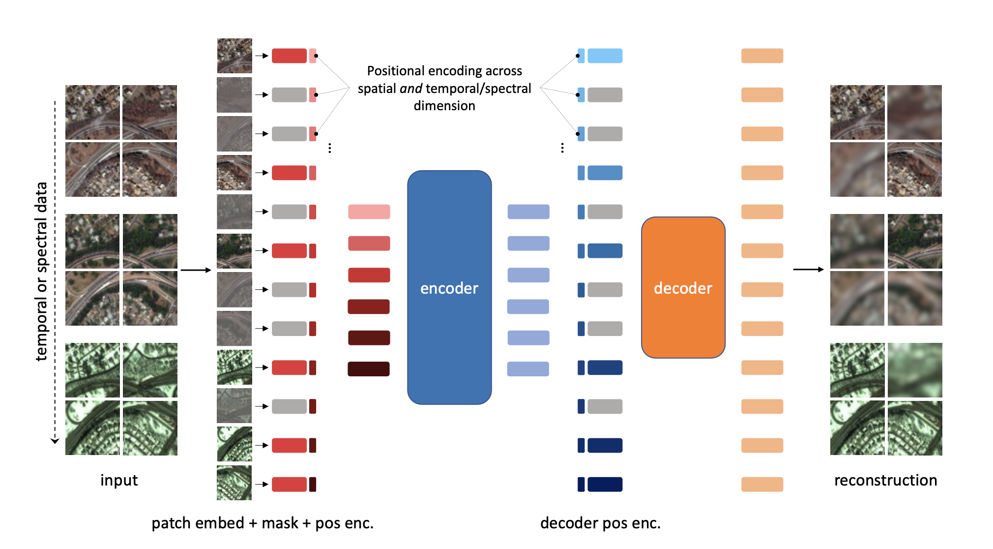
Foundation Model Architectures
Key architectures powering geospatial AI
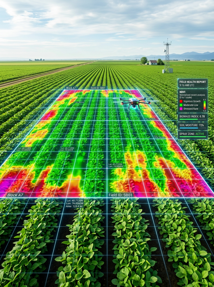
Agriculture: Crop Monitoring & Yield Prediction
Foundation models applied to precision agriculture
Crop type mapping using multi-temporal Sentinel-2 time series
Yield prediction by fusing remote sensing with weather and soil data
NDVI and vegetation index time-series modelling for phenology
Economically Optimal N Rate (EONR) mapping using ML
In-season nitrogen management with remote sensing at Z31 growth stage
Transfer learning enables model use across different fields and seasons
Agriculture: Soil Analysis & Experiment Design
Variable rate application and N-strip trial design
Platinum
Digital soil maps, yield maps, historical data
Satellite + ML
Full variable rate N application
Gold
Pre-season soil nutrients + plant phenology
Remote sensing + sensors
Zone-based management
Silver
PSA, CEC measurements
Electromagnetic induction
Basic zone mapping
Bronze
Yield map only
Standard GPS
Simple prescription maps
N-strip trials: three rates — low, normal, high — applied at Z31 growth stage
Machine learning predicts EONR based on seasonal rainfall, EM, remote sensing
Model transfers across fields and seasons for scalable precision agriculture
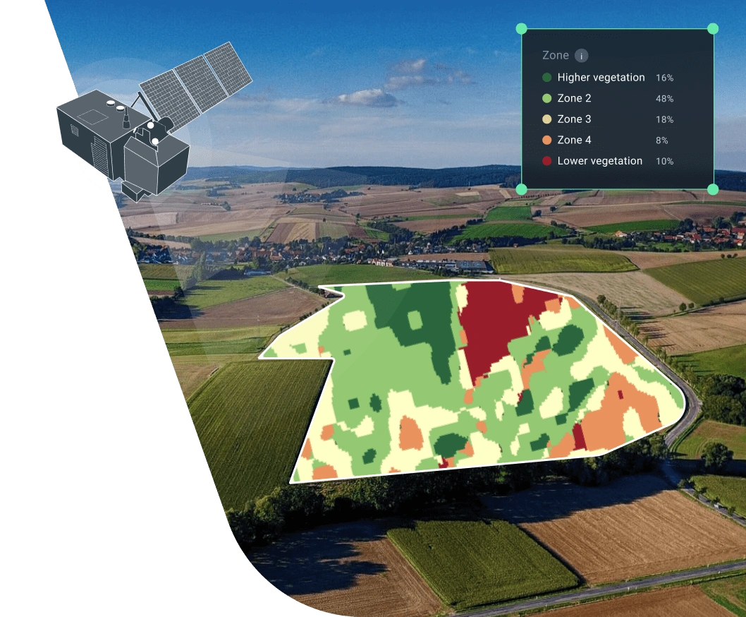
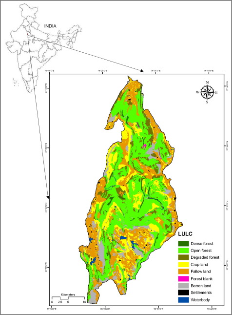
Environmental Applications
Land use, deforestation, flood and climate monitoring
Land Use and Land Cover (LULC) classification at continental scale
Deforestation and forest degradation monitoring using SAR time-series
Flood extent mapping: rapid response using Sentinel-1 SAR
Urban heat island detection and impervious surface mapping
Wetland and mangrove habitat monitoring with multispectral + LiDAR
Wildfire burn severity assessment using pre/post spectral indices
Drought stress monitoring via soil moisture and vegetation anomalies
Carbon stock estimation for ecosystem accounting
Key Foundation Models & Benchmarks
Overview of leading geospatial foundation models
Model
Developer
Architecture
Pre-training Data
Key Applications
Prithvi
NASA / IBM
ViT + MAE
HLS Landsat-Sentinel
Flood, crop, burn mapping
SatMAE
Caltech
MAE (temporal)
fMoW + Sentinel-2
Scene classification, detection
Clay
Clay Foundation
ViT + contrastive
Multi-sensor global
General geospatial tasks
GFM
Various
Swin Transformer
Multi-source RS
LULC, segmentation
RemoteCLIP
RSICD
CLIP (vision-language)
RS + captions
Image-text retrieval
Case Study: Prithvi Foundation Model
NASA and IBM — geospatial AI at scale
Developed by NASA and IBM, released as open-source in 2023
Pre-trained on 6 years of Harmonized Landsat-Sentinel (HLS) time-series data
100M parameter Vision Transformer with temporal positional encoding
Fine-tuned tasks: flood mapping, wildfire burn scar detection, crop segmentation
Achieves state-of-the-art on flood mapping with only 10% of labelled training data
Demonstrates strong transfer learning across geographic regions
Available on Hugging Face — enables community fine-tuning for new applications
Key lesson: foundation models dramatically reduce labelling burden in geospatial AI
Challenges and Limitations
Open problems in geospatial foundation models
Data heterogeneity:
sensors, resolutions, coordinate systems vary widely
Lack of large labelled benchmarks:
annotation is costly and expert-intensive
Generalisation across geographies:
models trained in one region may fail in another
Computational cost:
training and fine-tuning require significant GPU resources
Interpretability:
black-box nature complicates trust in high-stakes decisions
Temporal dynamics:
handling multi-year phenological cycles and climate shifts
Multi-modal fusion:
combining optical, SAR, LiDAR, and tabular data reliably
Ethical concerns:
data ownership, indigenous land data sovereignty, and bias
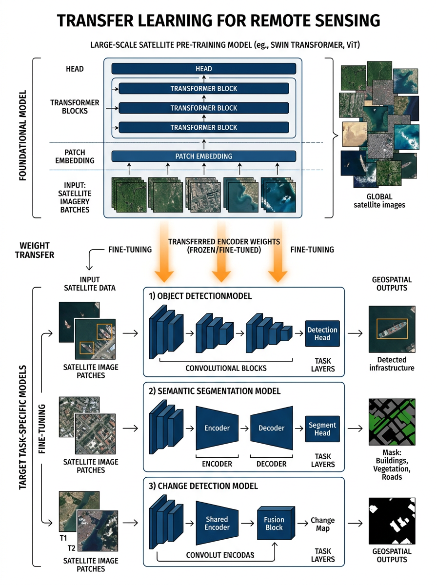
Transfer Learning & Fine-tuning
Adapting foundation models to new geospatial tasks
Fine-tuning: updating all or selected model weights on a labelled downstream dataset
Linear probing: freeze backbone, train only the classification head — fast and data-efficient
LoRA (Low-Rank Adaptation): inject small trainable matrices — reduces GPU memory requirements
Prompt tuning: condition the model using learnable task tokens — no weight updates needed
Domain adaptation: bridge spectral gap between training (Landsat/HLS) and target (Sentinel-2, MODIS)
Few-shot learning: achieve competitive performance with as few as 10–50 labelled samples
Cross-region transfer: models pre-trained in US/Europe applied to Australia, Africa, Southeast Asia
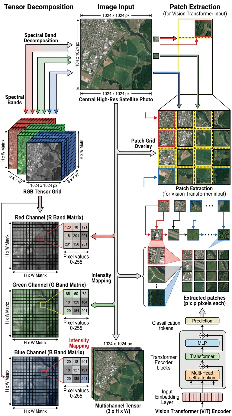
What an Image Is Mathematically
Pixels, channels, tensors, and from pixels to features
A digital image is a 3D tensor of shape H × W × C, where C = channels (e.g. 3 for RGB, 13 for Sentinel-2)
Each pixel holds intensity values in [0, 255] or normalised [0, 1] per channel
Colour images stacked as separate 2D matrices — red, green, blue each independent
Raw RGB pixels are not semantic: nearby pixels can belong to different classes
Local patterns (edges, textures) require filters — convolution extracts spatial features
Patches divide the image into fixed-size tiles (e.g. 16×16 px) — the input unit for transformers
What an Embedding Is
A learned vector z ∈ ℝᵈ that captures semantics
An embedding is a dense numerical vector that represents the meaning of an input, not just its pixels
Formally: z = f(x) where f is a neural network encoder and z ∈ ℝᵈ (e.g. d = 64, 256, 768)
Semantically similar inputs map to nearby vectors in the embedding space
Patch embeddings: each 16×16 image patch is linearly projected into a d-dimensional token
Tokenisation: the image becomes a sequence of N patch tokens, analogous to words in NLP
Embeddings carry richer information than raw pixel values — texture, shape, context
Latent Space
Geometry, neighborhoods, clustering, interpolation, semantic directions
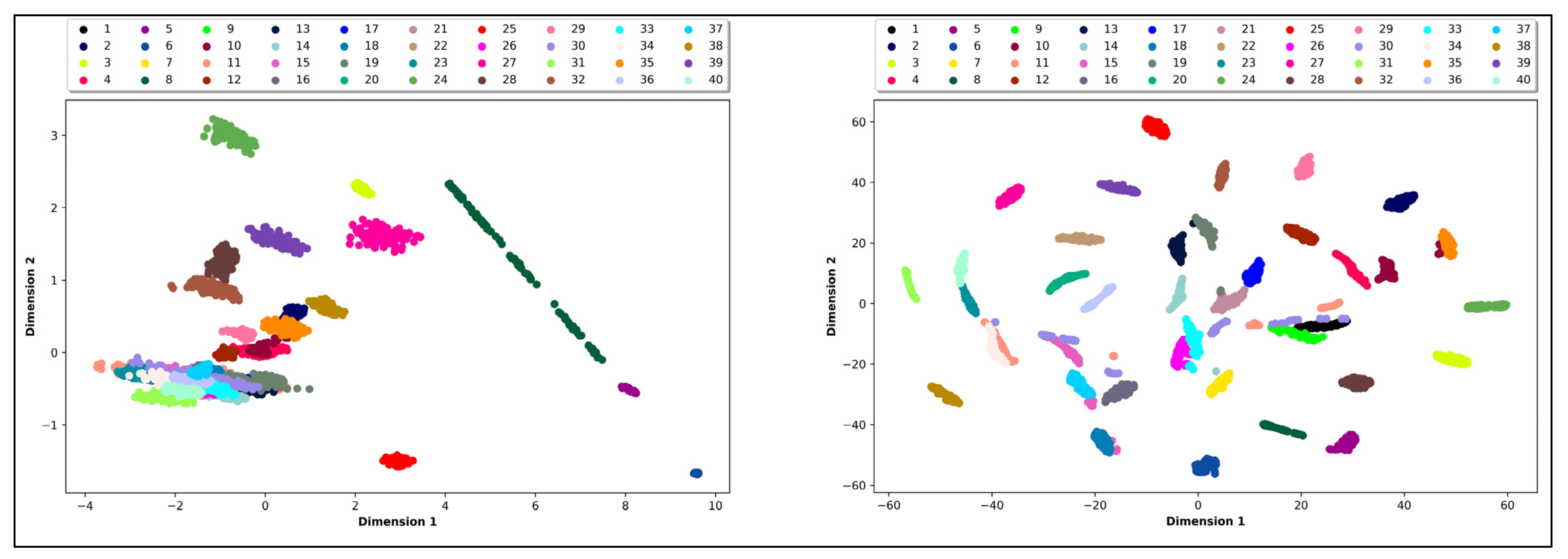
The latent space is the high-dimensional space where all embeddings live after encoding
Nearby points in latent space share semantic properties — e.g. 'forest' clusters together
Clustering: k-means or UMAP projections reveal meaningful groupings of land cover types
Interpolation: moving along a straight line between two embeddings smoothly transitions semantics
Semantic directions: PCA axes or learned directions encode concepts (e.g. 'more vegetation')
Well-structured latent spaces generalise better to unseen locations and sensor configurations
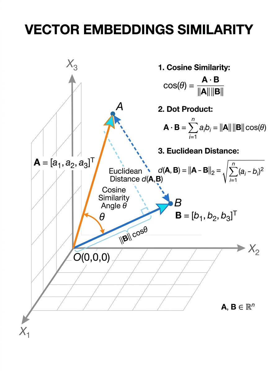
Similarity Math
Dot product, cosine similarity, Euclidean distance, nearest neighbours
<strong style="font-weight: bold;">Dot product:</strong> sim(a, b) = aᵀb — fast, used in attention mechanisms and retrieval
<strong style="font-weight: bold;">Cosine similarity:</strong> sim(a, b) = aᵀb / (‖a‖‖b‖) — measures angle, scale-invariant
<strong style="font-weight: bold;">Euclidean distance:</strong> d(a, b) = ‖a − b‖₂ — sensitive to magnitude, used in clustering
<strong style="font-weight: bold;">For unit-length embeddings</strong> (e.g. AlphaEarth): dot product equals cosine similarity
<strong style="font-weight: bold;">Nearest-neighbour search:</strong> find top-k most similar embeddings in large databases (FAISS)
<strong style="font-weight: bold;">Similarity enables zero-shot retrieval:</strong> find pixels/patches similar to a query without retraining
How Models Learn Embeddings
Supervised vs self-supervised objectives, contrastive learning, autoencoders
<strong style="font-weight: bold;">Supervised:</strong> learn embeddings using class labels — good performance, requires expensive annotations
<strong style="font-weight: bold;">Self-supervised:</strong> learn from data structure alone — no labels needed, scales to petabytes of satellite imagery
<strong style="font-weight: bold;">Contrastive learning:</strong> positive pairs (augmented views of same image) pulled together, negative pairs pushed apart
<strong style="font-weight: bold;">InfoNCE loss:</strong> maximise mutual information between positive pairs, foundational to MoCo and SimCLR
<strong style="font-weight: bold;">MoCo / SimCLR:</strong> seminal contrastive methods adapted for geospatial data (SeCo, GeoSSL)
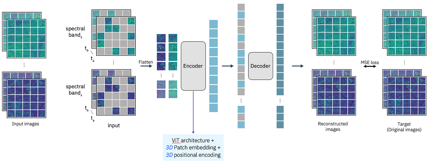
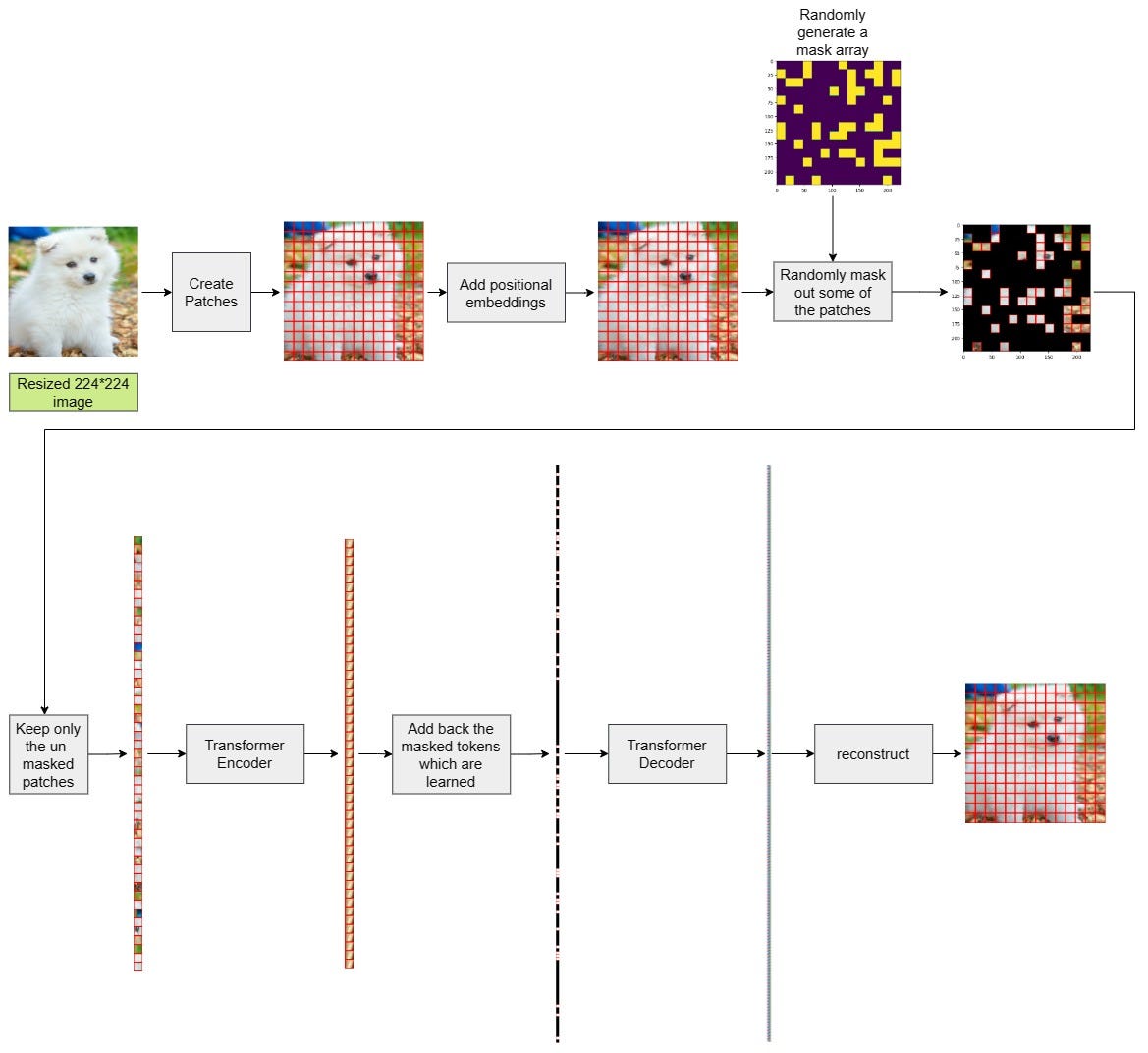
<strong style="font-weight: bold;">Autoencoders:</strong> compress input to bottleneck z, reconstruct output — forces z to capture essentials
<strong style="font-weight: bold;">MAE (Masked Autoencoder):</strong> mask 75% of patches, reconstruct — learns rich patch-level representations
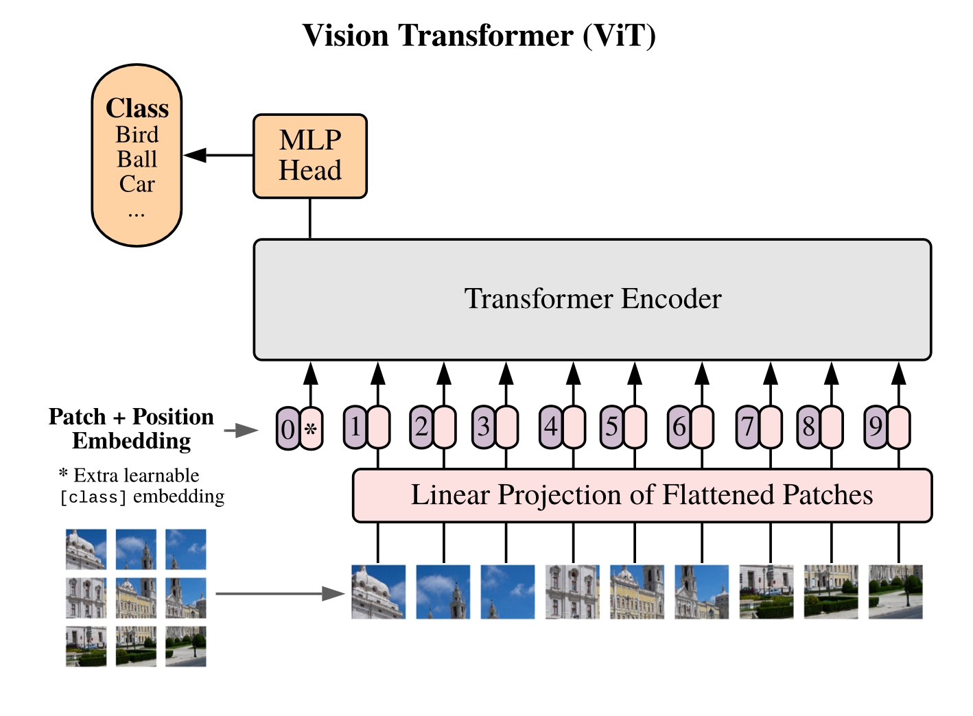
Transformers for Images
Self-attention, token mixing, and why ViTs changed embeddings
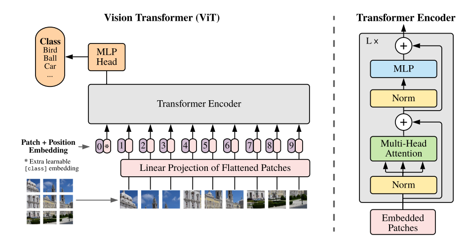
<strong style="font-weight: bold;">ViT (Vision Transformer):</strong> splits image into 16×16 patches, each projected to a token via linear embedding
<strong style="font-weight: bold;">Self-attention:</strong> each token attends to all others — captures global context unlike CNNs
<strong style="font-weight: bold;">Token mixing:</strong> information flows across the full image in every layer — long-range dependencies
<strong style="font-weight: bold;">Positional encodings:</strong> preserve spatial location of each patch token (learnt or Fourier-based)
<strong style="font-weight: bold;">ViT embeddings</strong> outperform CNN features on downstream remote sensing tasks with sufficient pre-training
<strong style="font-weight: bold;">Foundation models</strong> (Prithvi, SatMAE, Scale-MAE) all use ViT backbones pre-trained on satellite imagery
Remote Sensing Embeddings
Optical, SAR, temporal stacks, multi-modal fusion, pixel vs patch vs scene
<strong style="font-weight: bold;">Optical embeddings:</strong> derived from RGB or multispectral bands (Sentinel-2, Landsat) — sensitive to clouds
<strong style="font-weight: bold;">SAR embeddings:</strong> derived from radar backscatter — cloud-penetrating, captures structure and moisture
<strong style="font-weight: bold;">Temporal stack embeddings:</strong> multi-date image sequences encoded as a single vector capturing change over time
<strong style="font-weight: bold;">Multi-modal fusion:</strong> combine optical + SAR + LiDAR embeddings via concatenation or cross-attention
<strong style="font-weight: bold;">Pixel embeddings:</strong> one vector per pixel (e.g. AlphaEarth 64D at 10 m) — fine-grained spatial resolution
<strong style="font-weight: bold;">Patch embeddings:</strong> one vector per 16×16 tile — balance between detail and compute
<strong style="font-weight: bold;">Scene embeddings:</strong> one vector per full image chip — used for scene classification and retrieval
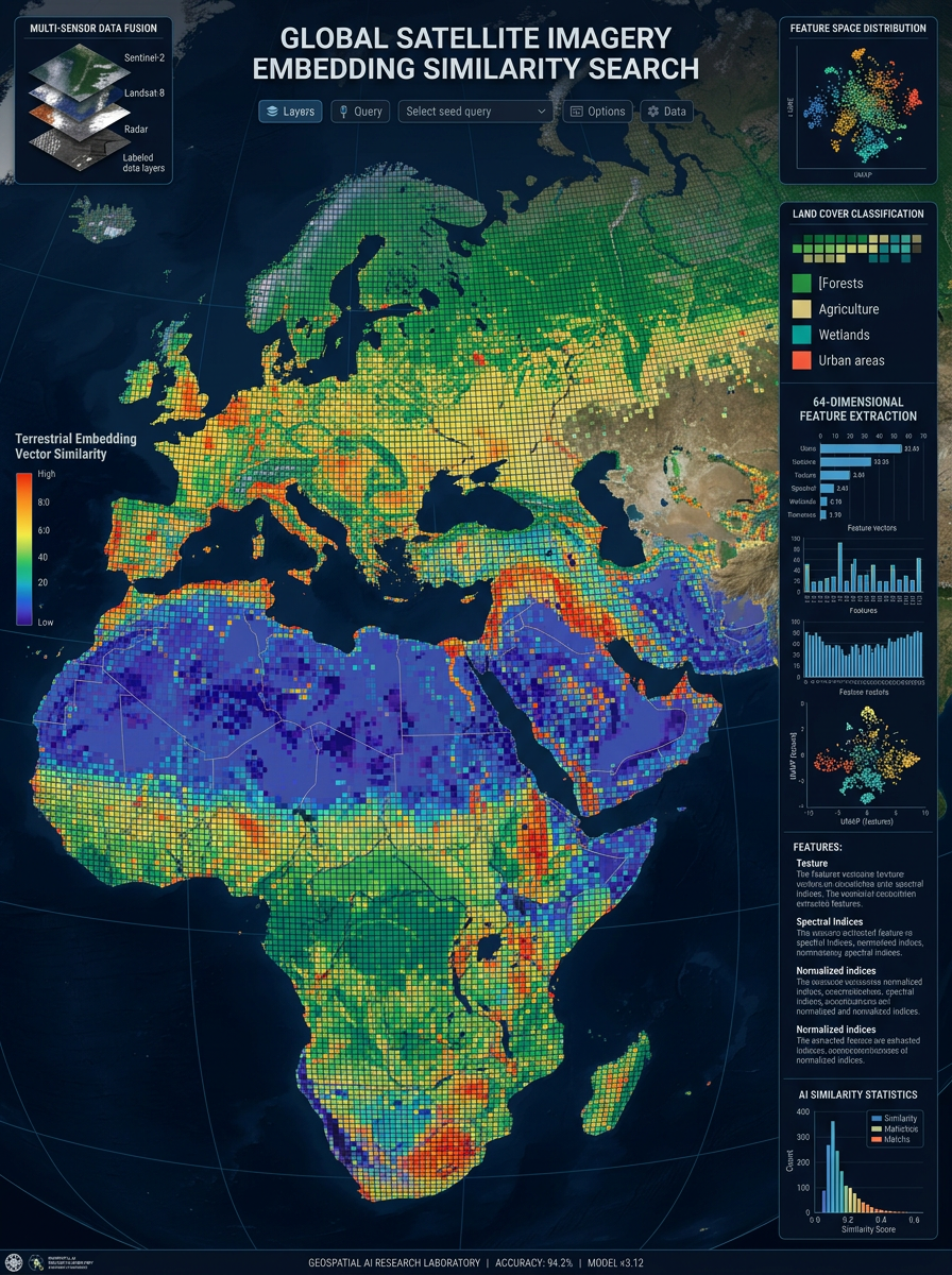
AlphaEarth Foundations — Case Study
A real geospatial embedding system at global scale
Annual 64-dimensional embeddings for every 10-metre pixel on Earth's land surface
Derived from multi-sensor yearly observations: Sentinel-2 optical + additional sensor stacks
Unit-length vectors: comparable across years via dot product or angle (cosine similarity = dot product)
Tasks supported: land cover classification, regression (e.g. yield, biomass), change detection, similarity search
Change detection: compare embedding angles between years — divergence = land use change
Similarity search: retrieve pixels globally that match a query location's embedding
Demonstrates the full pipeline: pixels → features → embeddings → latent space → downstream tasks
- geospatial-ai
- foundation-models
- remote-sensing
- precision-agriculture
- environmental-science
- machine-learning
- satellite-imagery
- nasa-prithvi