
Graph Coloring Theory & Chromatic Numbers Explained
Learn about graph coloring, the Four Color Theorem, greedy algorithms, and real-world applications like scheduling and register allocation.
Graph Theory • CS & Engineering
Graph Coloring, Chromatic<br>Numbers & the Four<br>Color Problem
An Introduction to Coloring Theory in Graph Theory
Undergraduate Graph Theory | Lecture Series
Table of Contents
What We'll<br>Cover Today
A step-by-step roadmap through the definitions, algorithms, theorems, and practical applications of graph coloring.
What is Graph Coloring?
Definitions & intuition
Chromatic Numbers
Measuring coloring efficiency
Greedy Coloring Algorithm
Step-by-step walkthrough
Special Graph Classes
Bipartite, planar, complete graphs
The Four Color Theorem
History & significance
Proving & Disproving Colorings
Tools & techniques
Real-World Applications
Maps, scheduling, compilers
What is Graph Coloring?
A <b>graph coloring</b> is an assignment of labels (called 'colors') to elements of a graph such that no two adjacent elements share the same color.
Imagine you're coloring a map — neighboring countries must always have different colors. Graph coloring is the mathematical version of this puzzle.
No two adjacent vertices may share the same color.
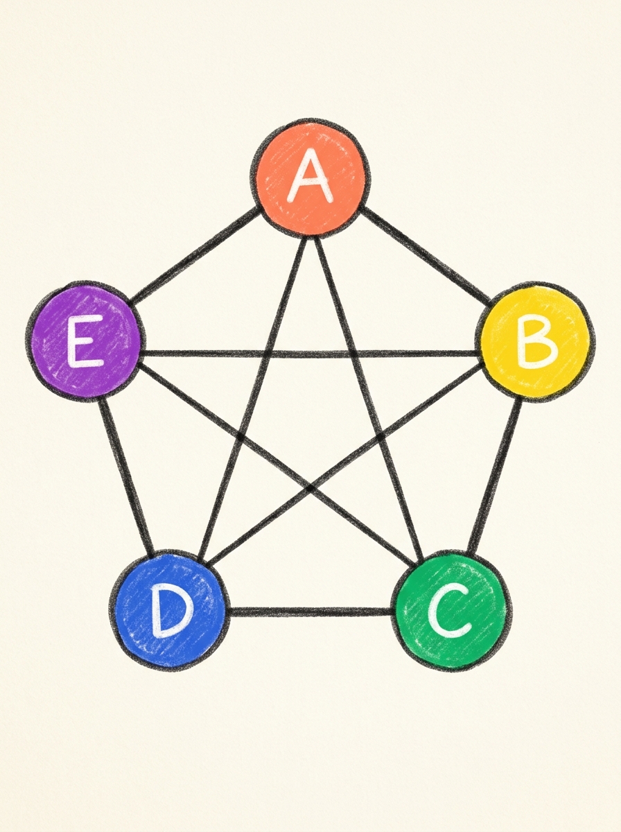
A valid 3-coloring of a simple graph
Worked Example: Coloring a Graph Step by Step
Draw the graph — 4 nodes: A, B, C, D. Edges: A-B, B-C, C-D, D-A, A-C
Start at node A — assign Color 1 (Red/Coral)
Move to B — adjacent to A, assign Color 2 (Green)
Move to C — adjacent to A and B, assign Color 3 (Blue). Move to D — adjacent to A and C, assign Color 2 (Green). Done!
✓ Valid 3-coloring achieved!
Try it yourself: can you color it with only 2 colors? Why not?
χ(G) = 3 for this graph
We used 3 colors and could not do it in 2.
Chromatic Numbers — χ(G)
Definition
minimum number of colors needed to properly color its vertices.
χ(G) = min colors for a valid coloring
It's not how many colors you CAN use — it's how few you NEED.
Key Values
χ(G) = 1
Graph has no edges (empty graph)
χ(G) = 2
Graph is bipartite
χ(G) = 3
Needs 3 colors (e.g., odd cycles)
χ(G) = n
Complete graph Kₙ
Graph Examples
P₄
χ = 2
K₃
χ = 3
K₄
χ = 4
Key Insight:
Finding χ(G) exactly is NP-hard in general — but we have powerful bounds and special cases!
Mention that chromatic number is a key graph invariant studied in combinatorics.
The Greedy Coloring Algorithm
How It Works
Order all vertices: v₁, v₂, ..., vₙ
(any order)
Assign the smallest available color to v₁
(Color 1)
For each next vertex vᵢ:
Look at all already-colored neighbors
Assign the smallest color NOT used by any neighbor
Repeat until all vertices are colored
Time Complexity: O(V + E)
Does NOT always find χ(G)
Result depends on vertex ordering!
Worked Trace on C₅ Graph
A greedy trace on a cycle C₅ — result: 3 colors (but χ(C₅)=3 ✓)
Greedy may use more colors than optimal. For C₅, it matches χ — but this isn't always guaranteed.
Special Graph Classes & Their Chromatic Numbers
Complete Graph Kₙ
χ(Kₙ) = n
Every pair adjacent → every node needs unique color
Bipartite Graph
χ = 2
Two sides, no intra-side edges → just 2 colors suffice
Cycle Cₙ (even)
χ = 2
Even cycles are bipartite → 2-colorable
Cycle Cₙ (odd)
χ = 3
Odd cycles force a third color — can you see why?
Tree
χ = 2
Trees are bipartite — always 2-colorable
Planar Graph
χ ≤ 4
The Four Color Theorem guarantees this!
Pattern: The more connections a graph has, the more colors it needs.
The Four Color Theorem
Every Planar Map Can Be Colored with Just 4 Colors
The Statement
Any map drawn on a plane can be colored using at most 4 colors such that no two adjacent regions share the same color.
1852
Francis Guthrie first poses the problem while coloring a map of England
1879
Alfred Kempe publishes a 'proof' (later found flawed)
1890
Percy Heawood shows Kempe's proof has a gap
1976
Appel & Haken finally prove it — using a computer for the first time in math history!
1997
Robertson et al. produce a cleaner computer-assisted proof
The Four Color Theorem was the first major theorem proved using a computer.
A 4-colored planar map — no two bordering regions share a color
Why Is It So Hard to Prove?
The Challenge
You can't just check examples — there are infinitely many possible planar graphs.
A valid proof must work for ALL planar maps, not just specific ones.
Kempe's Flawed Proof (1879)
Alfred Kempe introduced 'Kempe chains' — swapping color sequences to free up a color slot.
His argument worked for most cases... but Percy Heawood found a specific graph in 1890 where it failed.
The flaw: Kempe assumed two separate chain swaps were independent — they weren't.
Appel & Haken's Breakthrough (1976)
Reduced ALL planar graphs to 1,936 'unavoidable configurations'.
Used a computer to verify each configuration — took 1,200 hours of CPU time!
Controversial at first: "Can we trust a proof a human can't fully read?"
Appel & Haken's Strategy: Reduce to finite cases
Every planar graph contains at least one of these unavoidable configurations.
The proof exists, but no simple human-readable proof has been found yet.
Bounding the Chromatic Number
Lower Bounds
χ(G) ≥ ω(G)
The clique number <strong style="color: #E8533F;">ω(G)</strong> is the size of the largest complete subgraph (clique). You need at least as many colors as the size of the largest clique.
If G contains K₄ (4 mutually adjacent nodes) → χ(G) ≥ 4
Upper Bounds
χ(G) ≤ Δ(G) + 1
<strong style="color: #2E7D32;">Δ(G)</strong> is the maximum degree (most edges at any single node). Brooks' Theorem: χ(G) ≤ Δ(G) for most graphs (except complete graphs and odd cycles).
If max degree = 3, then χ(G) ≤ 4 (or often ≤ 3 by Brooks)
clique lower bound
ω(G)
χ(G)
Δ(G) + 1
degree upper bound
The gap between ω(G) and χ(G) can be arbitrarily large — Mycielski graphs have χ → ∞ but ω = 2!
Real-World Applications
Map Coloring
Color regions of a geographic map so no two adjacent countries/states share a color. The classic motivation for the Four Color Theorem.
Exam / Job Scheduling
Represent exams as nodes; connect exams with shared students. Coloring gives a conflict-free schedule — colors = time slots.
Compiler Register Allocation
Variables in a program are nodes; connect those that conflict (live at same time). Colors = CPU registers. Minimize registers used.
Frequency Assignment
Mobile towers are nodes; edges = overlapping coverage areas. Colors = radio frequencies. Prevent signal interference.
Sudoku Solving
A 9×9 Sudoku grid is a graph where cells in the same row/col/box are adjacent. Solving = graph coloring with χ = 9.
Chemical Storage
Chemicals are nodes; edges = dangerous if stored together. Colors = storage rooms. Minimize rooms while preventing reactions.
Graph Coloring turns real-world conflict problems into elegant mathematical ones.
Deep Dive: Exam Scheduling with Graph Coloring
The Problem Setup
A university has 5 exams: Math, Physics, CS, Chemistry, History. Some students are enrolled in multiple courses. Exams with shared students CANNOT be scheduled at the same time.
Math–Physics, Math–CS, Physics–Chemistry, CS–Chemistry, Chemistry–History, History–Math
Step 1: Build the conflict graph
nodes = exams, edges = conflicts
Step 2: Color the graph
use greedy coloring:
<b>Math</b> → Slot 1 <span style="color:#888888; font-size: 20px;">(coral)</span>
<b>Physics</b> → conflicts with Math → Slot 2 <span style="color:#888888; font-size: 20px;">(green)</span>
<b>CS</b> → conflicts with Math → Slot 2 <span style="color:#888888; font-size: 20px;">(green)</span> <span style="font-size: 18px;">[no conflict with Physics]</span>
<b>Chemistry</b> → conflicts with Physics, CS → Slot 3 <span style="color:#888888; font-size: 20px;">(blue)</span>
<b>History</b> → conflicts with Chemistry, Math → Slot 2 <span style="color:#888888; font-size: 20px;">(green)</span>
Result: 3 time slots needed — χ(G) = 3!
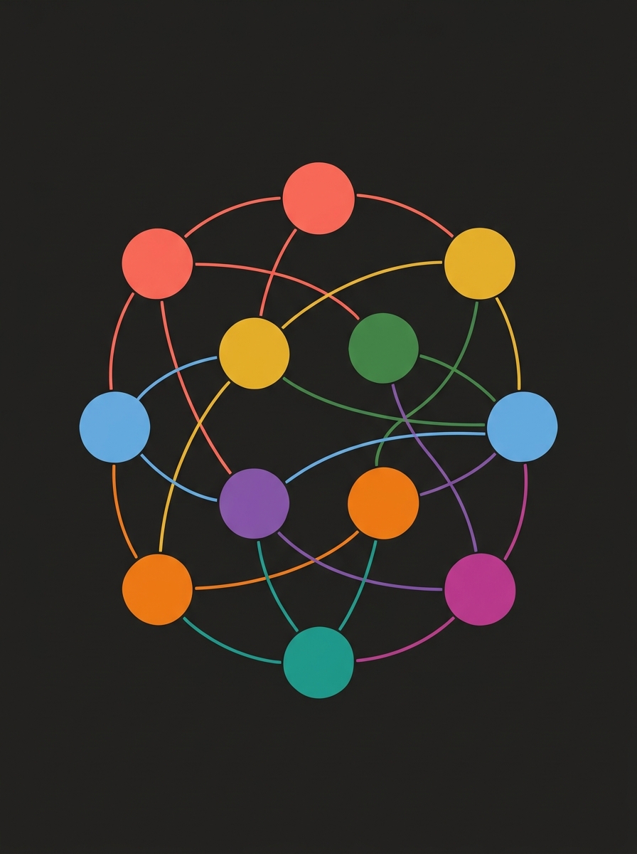
The Graph Visualization
This approach is used by real universities and software tools for automated scheduling!
How Hard Is Graph Coloring?
Complexity Results
2-Coloring (Bipartite Check)
Solvable in O(V+E) time using BFS/DFS. Check if graph is bipartite — if yes, χ=2.
✓ Polynomial — Easy!
3-Coloring
Determining if χ(G) ≤ 3 is NP-Complete. No efficient algorithm is known for all graphs.
✗ NP-Complete — Hard!
k-Coloring (k ≥ 3)
For any fixed k ≥ 3, deciding if χ(G) ≤ k is NP-Complete.
✗ NP-Complete — Hard!
Approximation
We can approximate χ(G) within a factor, but not arbitrarily close unless P=NP.
The Big Picture: Graph coloring is one of Karp's original 21 NP-complete problems (1972).
Efficient algorithms exist for special graph classes — trees, planar graphs, interval graphs — even if the general problem is hard.
Key Insight: Knowing a graph's structure (planar, bipartite, sparse) unlocks faster solutions.
SUMMARY
Key Takeaways
Graph coloring assigns colors to vertices so no two adjacent vertices share a color
The chromatic number χ(G) is the minimum colors needed
Greedy coloring is simple but may not find the optimal χ(G)
Bipartite graphs: χ=2. Odd cycles: χ=3. Complete graphs: χ=n
The Four Color Theorem: every planar map needs at most 4 colors
Graph coloring solves scheduling, register allocation, frequency assignment & more
What's Next?
Edge Coloring & Vizing's Theorem
List Coloring & Choosability
Fractional Chromatic Numbers
Graph Coloring Algorithms & Approximation
Undergraduate Graph Theory | Lecture Series
Thank You!
Questions?
- graph-theory
- chromatic-numbers
- four-color-theorem
- computer-science
- algorithms
- discrete-mathematics
- scheduling